I. Experimental Scenario: Study on Morphological‑Distribution Characteristics of Brain Neurons in Fly Heads of Different Sizes

In this study, adult Drosophila melanogaster was selected as the experimental model for its remarkable advantages in investigating the morphology and distribution of brain neurons. First, the nervous system of adult flies is fully developed with mature and stable brain structures and neural circuits, which can accurately reflect neuronal‑distribution features of adults and eliminate phenotypic interference caused by dynamic development at larval or pupal stages. Second, commonly‑used laboratory fly strains feature stable genetic backgrounds and uniform phenotypes, ensuring highly repeatable experimental results. In addition, the adult‑fly brain is small‑sized with a relatively simple structure. Combined with a confocal microscope, rapid whole‑brain imaging and 3D reconstruction can be achieved, facilitating clear visualization of overall neuronal projection patterns.

Meanwhile, well‑established genetic manipulation techniques in flies (e.g., GAL4/UAS system) enable specific labelling of distinct neuronal subpopulations, providing powerful technical support for precise analysis of neuronal morphology and distribution. Overall, adult fruit‑flies are an ideal classic model for studying brain‑neuron morphology and distribution, featuring low breeding costs, short reproduction cycles, minimal ethical requirements and easy sample‑size control.

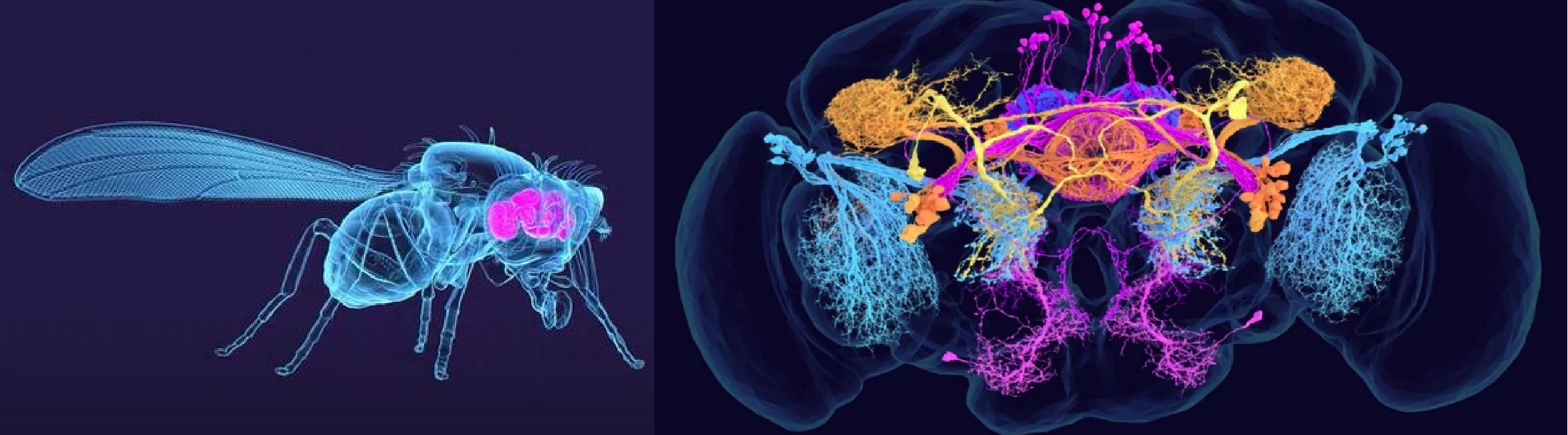
Figure 1: Whole‑brain view of adult Drosophila

The morphology and distribution of neurons in the Drosophila brain reflect high efficiency, modular organization and functional specificity. Morphological characteristics of neurons (1) Small size and limited quantity (2) Highly specialized morphological features (3) Highly conserved circuit architecture

Distribution characteristics of neurons (1) Layered and modular structure (2) Bilateral symmetry and cross‑connectivity (3) Specific distribution of neurotransmitter/neuromodulator systems

In this experiment, laser‑scanning confocal microscopy was applied to observe the morphology and structure of neuronal synapses in fly heads of different sizes (10 mm, 30 mm), so as to analyze their functional‑regulation mechanisms within the nervous‑system network. Both macro‑ and micro‑morphological observations were carried out on the morphology and distribution of neurons in fruit‑fly brains of varying sizes.

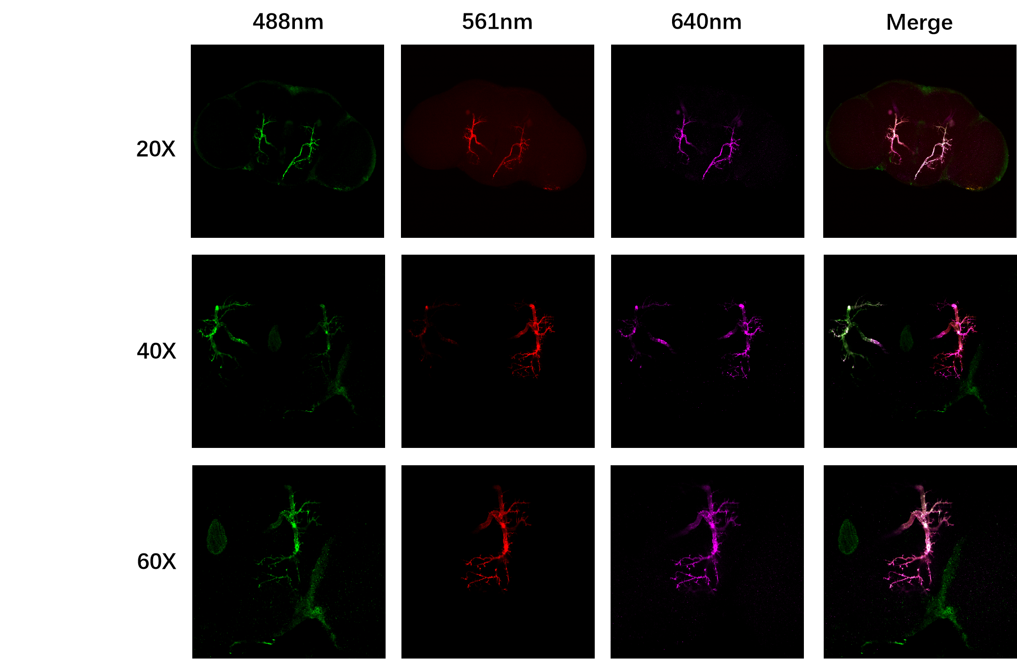
Synapses act not only as relay stations for neural signals, but also as intelligent processors for information processing, storage and adaptive modification. The molecular mechanisms and plasticity of synapses are highly conserved in model organisms such as Drosophila, which is of great significance for understanding brain function and developing therapies for brain‑related diseases. In this experiment, the NCF1000 laser confocal microscope was used for observation under 20×, 40× and 60× objectives. Neuronal morphological features were characterized through combined macro‑ and micro‑scale imaging.

Figure 2: Imaging acquisition parameters

Microscope: NCF1000 Laser Scanning Confocal Microscope Objectives: 20× (N.A. = 0.75), 40× (N.A. = 0.95), 60× (N.A. = 1.42, Oil) Resolution: 2048 × 2048 pixels Laser channels: 488 nm (GFP), 561 nm (Hemagglutinin tag, YPYDVPDYA), 640 nm (V5 tag‑SV5 Pk epitope, GKPIPNPLLGLDST) Function: Multi‑channel confocal image fusion

During whole‑brain imaging, the MCFO (Multi‑Color FlpOut) technique was adopted for multi‑colour neuronal tracing. Adjacent neurons are labelled with different colours, which helps visualize cell boundaries, trace neuronal projections and identify co‑localization or signal overlap. With the NCF1000 confocal microscope, users can clearly resolve the morphology and location of fluorescent markers across channels at different magnifications, characterize neural‑circuit performance and further explore the relationship between neurons and animal behaviours.

II. How the NCF1000 Confocal Microscope Supports This Experiment

1. Z‑Stack Acquisition

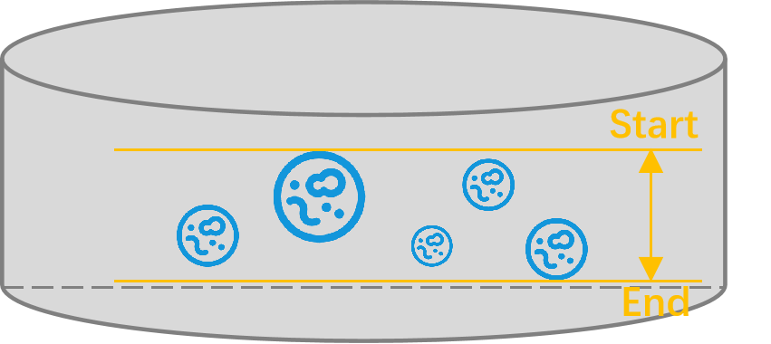
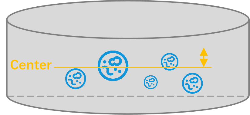
Z‑stack images are acquired for 3D reconstruction. Two acquisition modes are available: Start/End mode and Center mode. ‑ In Start/End mode, users define the upper and lower boundaries to set the Z‑axis range for 3D imaging (Figure 7). ‑ In Center mode, users specify the mid‑point of the Z‑axis and the desired 3D thickness to determine the imaging volume (Figure 8). This function enables researchers to capture precise 3D structural information of specimens and improve imaging resolution and detail.

Z‑stack acquisition can be performed via the supporting software NomisPro X‑C (on‑line acquisition) or the offline software NomisPro X‑V.

Figure 6: Schematic diagram of Z‑Stack Start/End‑mode interface

Figure 7: Schematic diagram of Z‑Stack Center‑mode interface

2. 3D Visualization Function

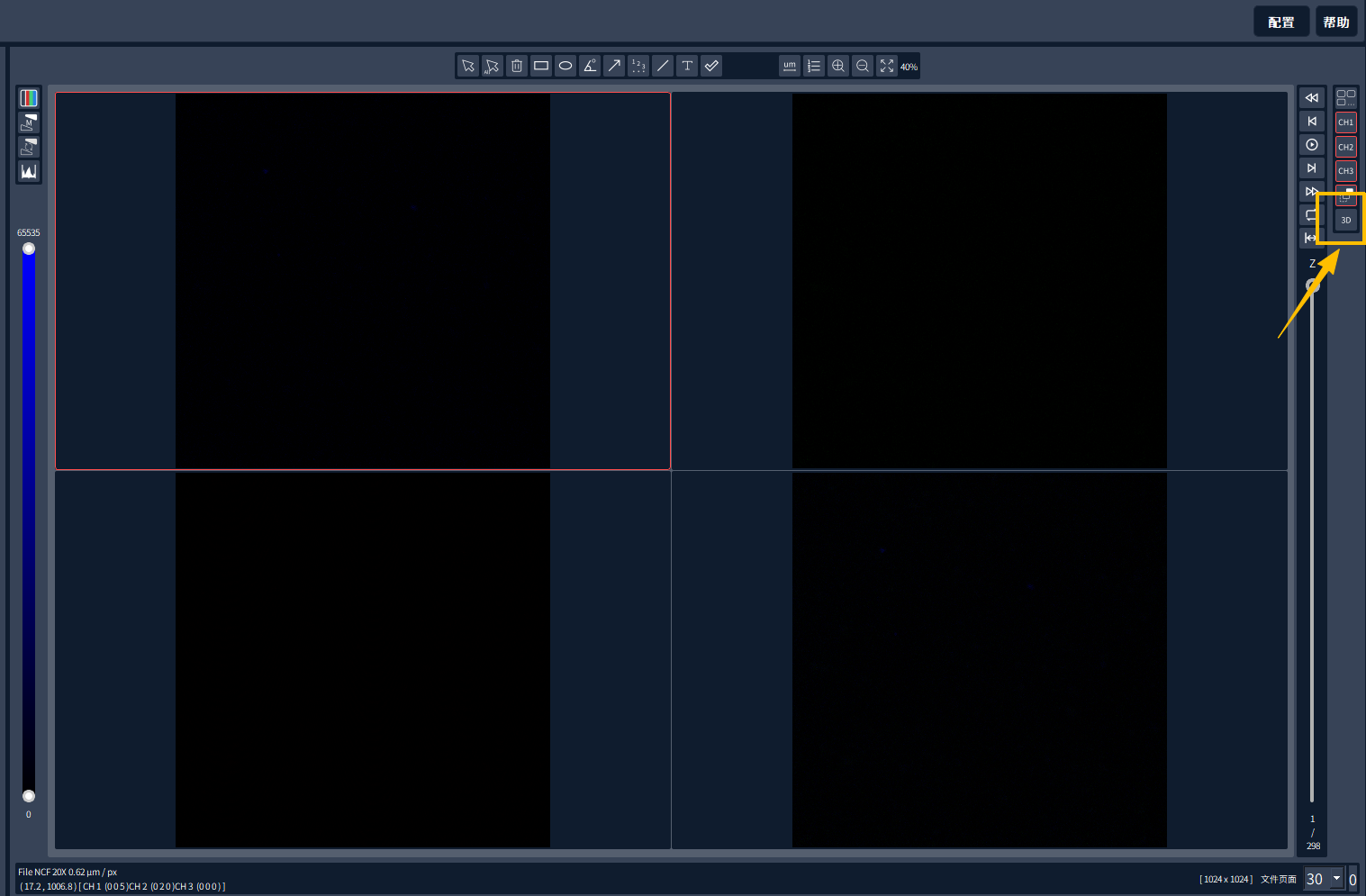
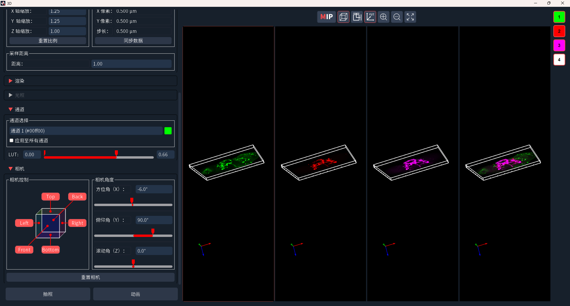
The 3D‑display function renders a 3‑dimensional model from a series of 2‑dimensional Z‑stack slices. After importing Z‑stack images into NomisPro X‑C or offline NomisPro X‑V, users can trigger 3‑D rendering with one click to generate reconstructed models (Figure 8). On the 3‑D viewer interface, channel‑specific histogram adjustments can be performed, and 3‑D models can be viewed from multiple perspectives (Figure 9).

Figure 8: 3D‑image display entry interface

Figure 9: 3D visualization and adjustment interface

III. Frequently‑encountered Experimental Issues & Answers

Q1: Can partial 3‑D imaging be performed while rendering full‑volume 3‑D reconstructions? A1: The NCF1000 confocal microscope supports standard multi‑channel volumetric Z‑stack scanning and full‑volume 3‑D rendering. Partial‑region 3‑D imaging is not currently available.

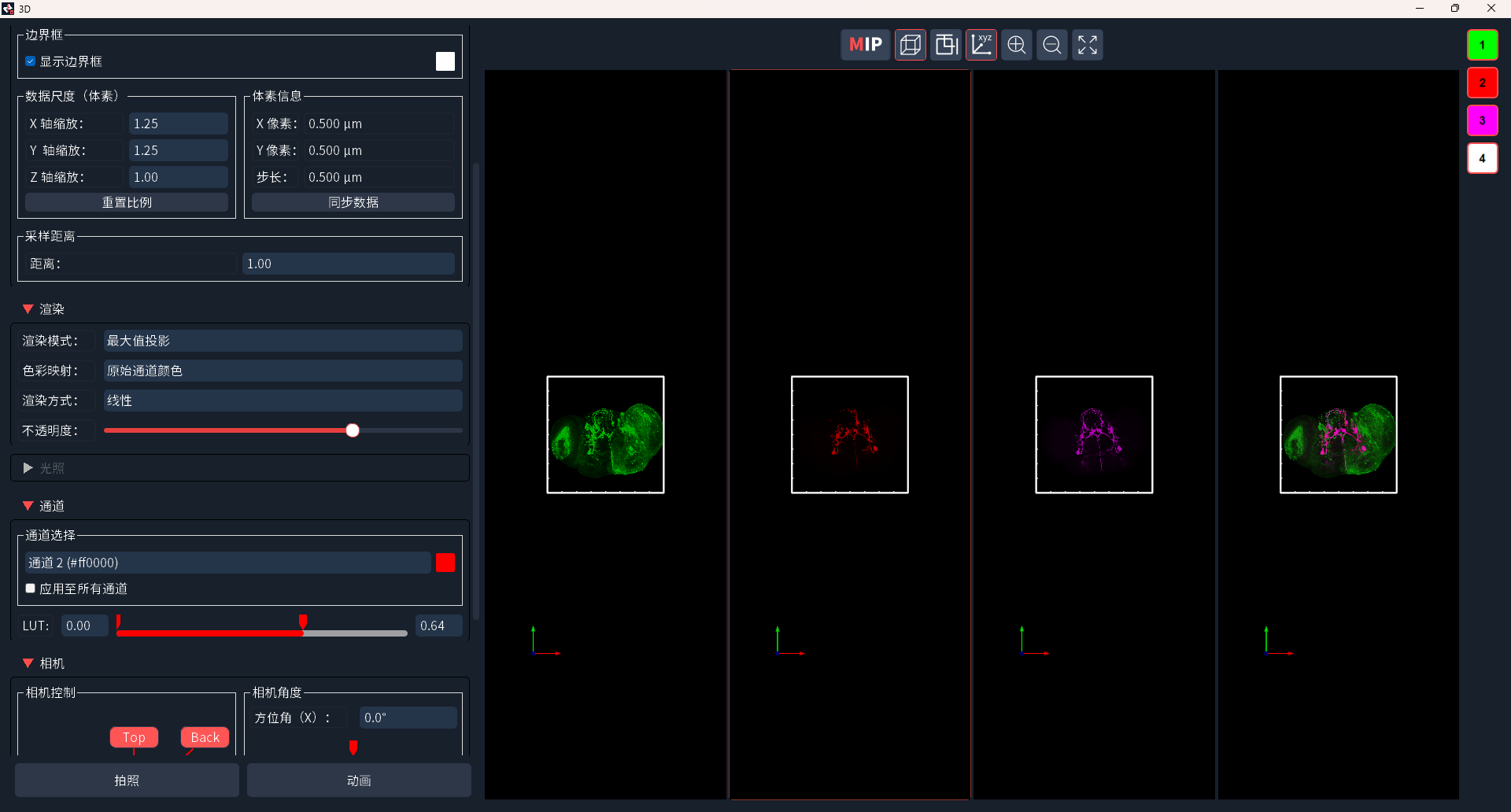
Q2: Can I adjust the histogram scale independently for each channel during 3‑D observation? A2: Import volumetric scanning data into the offline software NomisPro X‑V and click the 3D button on the right‑hand panel to launch 3‑D visualization. Histogram values can then be adjusted for individual channels, and the resulting images or videos can be exported.

Figure 10: Interface for channel‑specific histogram adjustment under 3‑D view